Towards a weakly nonlinear nonmodal stability theory

As briefly introduced in the “ Linear modal and nonmodal stability ” page of this website, the Navier-Stokes operator linearised around a nonzero background flow is frequently non-normal. In that case, the linear flow response to an external perturbation can be spanned by a generically vast number of nonorthogonal eigenmodes (nonorthogonal under the same inner product as that used to compute the adjoint operator). Accordingly, the corresponding induced norm of the response can take substantial values, resulting from the interactions between these numerous eigenmodes.

Let us make this statement more precise. If \(\{q_j \}_{j\geq 1}\) and \(\{q^{\dagger}_j \}_{j\geq 1}\) designate the direct and adjoint eigenmodes family of the linearised operator, respectively, and associated with the eigenvalues \(\{\sigma_j \}_{j\geq 1}\), then the linear response \(\hat{u}_h \exp{(i \omega_o t)} + c.c.\) to a harmonic forcing \(\hat{f}_h \exp{(i \omega_o t)} + c.c.\) is such that

\[\hat{u}_h = R(\omega_o) \hat{f}_h = \sum_j \frac{ q_j }{i\omega_o - \sigma_j} \frac{\langle q^{\dagger}_j \mid \hat{f}_h \rangle}{ \langle q^{\dagger}_j \mid q_j \rangle },\]

where \(R(\omega_o)\) is the resolvent operator. Thereby,

\[\left\| \hat{u}_h \right\|^2 = \sum_j \frac{ \left\| q_j \right\|^2 }{\left| i\omega_o - \sigma_j \right|^2} \frac{\left| \langle q^{\dagger}_j \mid \hat{f}_h \rangle \right|^2}{\left| \langle q^{\dagger}_j \mid q_j \rangle \right|^2 } + \sum_j \sum_{k\neq j} \frac{ \langle q_j \mid q_k \rangle }{(i\omega_o - \sigma_j)^*(i\omega_o - \sigma_k)} \frac{\langle q^{\dagger}_j \mid \hat{f}_h \rangle^* \langle q^{\dagger}_k \mid \hat{f}_h \rangle }{\langle q^{\dagger}_j \mid q_j \rangle^* \langle q^{\dagger}_k \mid q_k \rangle},\]

where the star denotes the complex conjugate. Now, if the linearised operator is non-normal, then remember that the eigenmodes do not form an orthogonal set. Consequently, the double sum term in the expression above, which involves eigenmode-eigenmode interactions through the inner product \(\langle q_j \mid q_k \rangle\), has no reason to vanish if \(\hat{f}_h\) projects over more than one adjoint mode (which is generically the case) ! In other words, the energy of the harmonic response, \(\left\| \hat{u}_h \right\|^2\), is determined by a possibly enormous number of eigenmode-eigenmode interactions. The eigenmodes thus form a very inefficient basis, in the sense that the harmonic response is inefficiently described by a single or even a few of them!

That is why these responses are said to be “ nonmodal ” : to insist on the inefficiency of the eigenbasis to describe them.

Nevertheless, in the previous page, the developments and conclusions were within the framework of linear dynamics, exact only in the limit of infinitesimal perturbations. However, even if a perturbation is small enough for the linearization to be valid at initial times, precisely because its response can be substantially amplified through linear non-normal mechanisms, the nonlinear interactions of the latter may not remain negligible! These latter typically modify the linear responses , as represented in figure 1.

Figure 1. Cartoon representation of nonlinearity and non-normality, illustrated in the time domain (a) and frequency domain (b), for a linearly stable system; the least stable eigenvalue \( \sigma_1 \) of the eigenspectrum in (c) indeed has a negative growth rate. (a) In the linear regime, the amplitude of the perturbations eventually decays like \( \exp{( \sigma_{1,r} t)} \). Non-normal systems can experience a very large transient growth. Nonlinearity may be stabilising or destabilising. (b) Normal systems subject to external forcing respond preferentially at frequency \( \sigma_{1,i} \). Non-normal systems can respond at different frequencies, with an amplification much larger than predicted by \( \sigma_{1,r} \). Nonlinearity may be stabilising or destabilising.

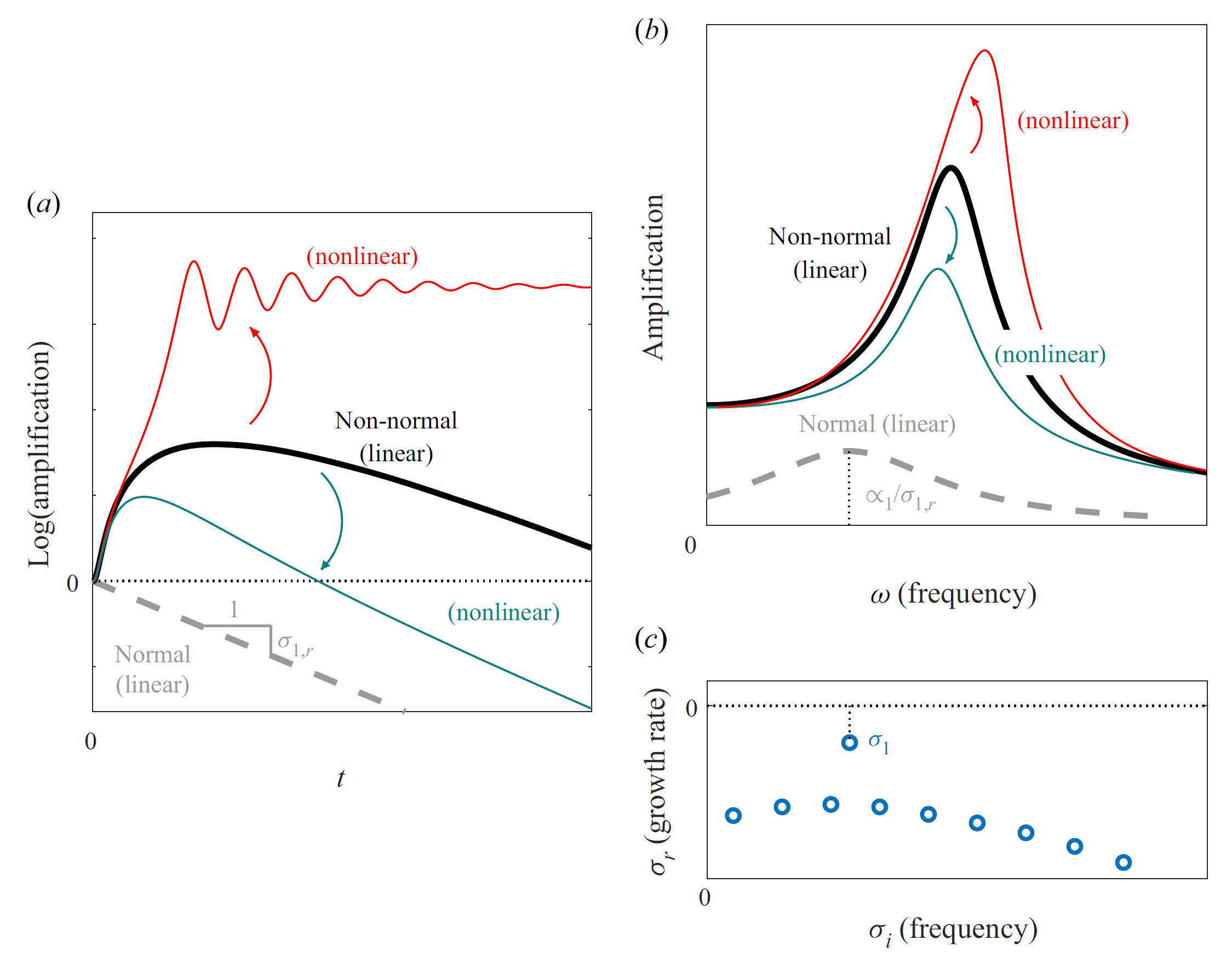
This calls for the study of nonlinear effects on nonmodal flow responses, which was the topic of my Ph.D. thesis (Ducimetière, 2024).

In doing so, the first step was to notice that nonmodal tools, solving for the maximum possible response-to-forcing amplification (typically by performing a svd decomposition), makes it possible to construct an orthonormal basis for the structure of the flow excitation and its response. The respective contribution to the induced norm of the response of each element of this basis can then be prioritized according to its associated (scalar) “ gain ”. For these reasons, as well as the orthonormality property, these new bases are much more efficient than the direct and adjoint eigenmodes bases.

Considering anew the harmonic response as an example, the latter can be rewritten

\[\hat{u}_h = \sum_{j} G_j \check{u}_j \langle \check{f}_j \mid \hat{f}_h \rangle,\]

where the pair \((\check{u}_j,\check{f}_j)\) is the \(j\)th singular modes pair of the resolvent operator \(R(\omega_o)\), normalized as \(\left\| \check{u}_j \right\| = \left\| \check{f}_j \right\| = 1\) for every \(j\geq 1\). The scalar \(G_j\) is the associated gain, such that \(G_j\check{u}_j = R(\omega_o)\check{f}_j\). Both the \(\{ \check{u} \}_{j\geq 1}\) and \(\{\check{f} \}_{j\geq 1}\) families have the desired property to be orthonormal, such that \(\left\| \hat{u}_h \right\|\) is now much more simply expressed

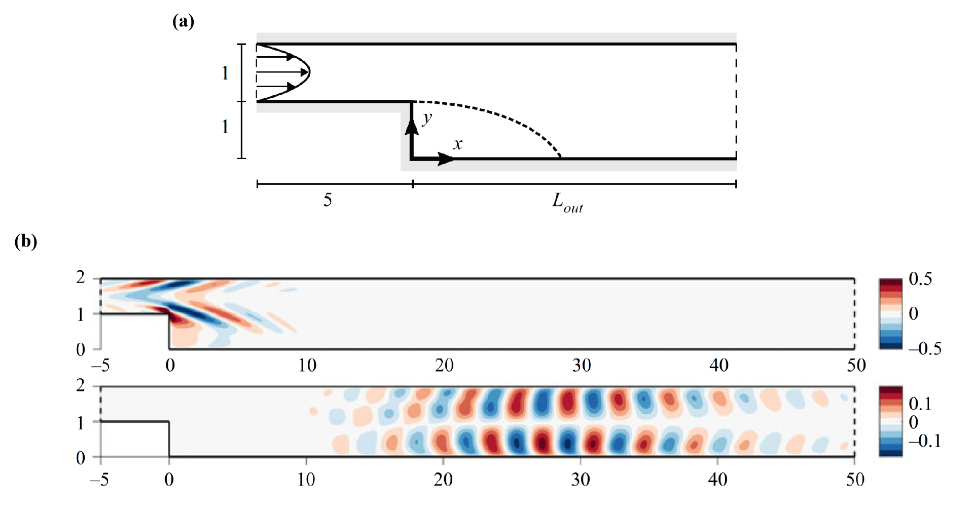
\[\left\| \hat{u}_h \right\|^2 = \sum_j G^2_j \left| \langle \check{f}_j \mid \hat{f}_h \rangle \right|^2.\]

Crucially, in fluid Mechanics, it is often the case that the responses to only a few of these forcing structures dominate the linear response, a property referred to as the low-rank approximation . We refer to figures 2 and 3 for an example.

Figure 2. (a) Sketch of the two-dimensional flow over a backward-facing step (BFS), with a fully developed parabolic profile of unit maximum centreline velocity at the inlet. (b) Corresponding streamwise (\( x \)) component of the optimal harmonic forcing structure \( Re(\hat{f}_1) \) at \( Re=500 \) and at the optimal forcing frequency \( \omega_o = 0.47 \) (top), and streamwise component of the associated response \( Re(\hat{u}_1) \) (bottom).

Figure 3. For the BFS flow sketched in Fig. 2. and at \( Re=500 \) Top: optimal linear harmonic gain \(G_1\) (full line). The first suboptimal gain \(G_2\) is also reported as the dashed-dotted line. Gains are shown as a function of the forcing frequency. Bottom: spectrum of this same flow in the complex plane (each dot an eigenvalue). The frequency ranges on the \(x\)-axis are the same for both the top and the bottom frames.

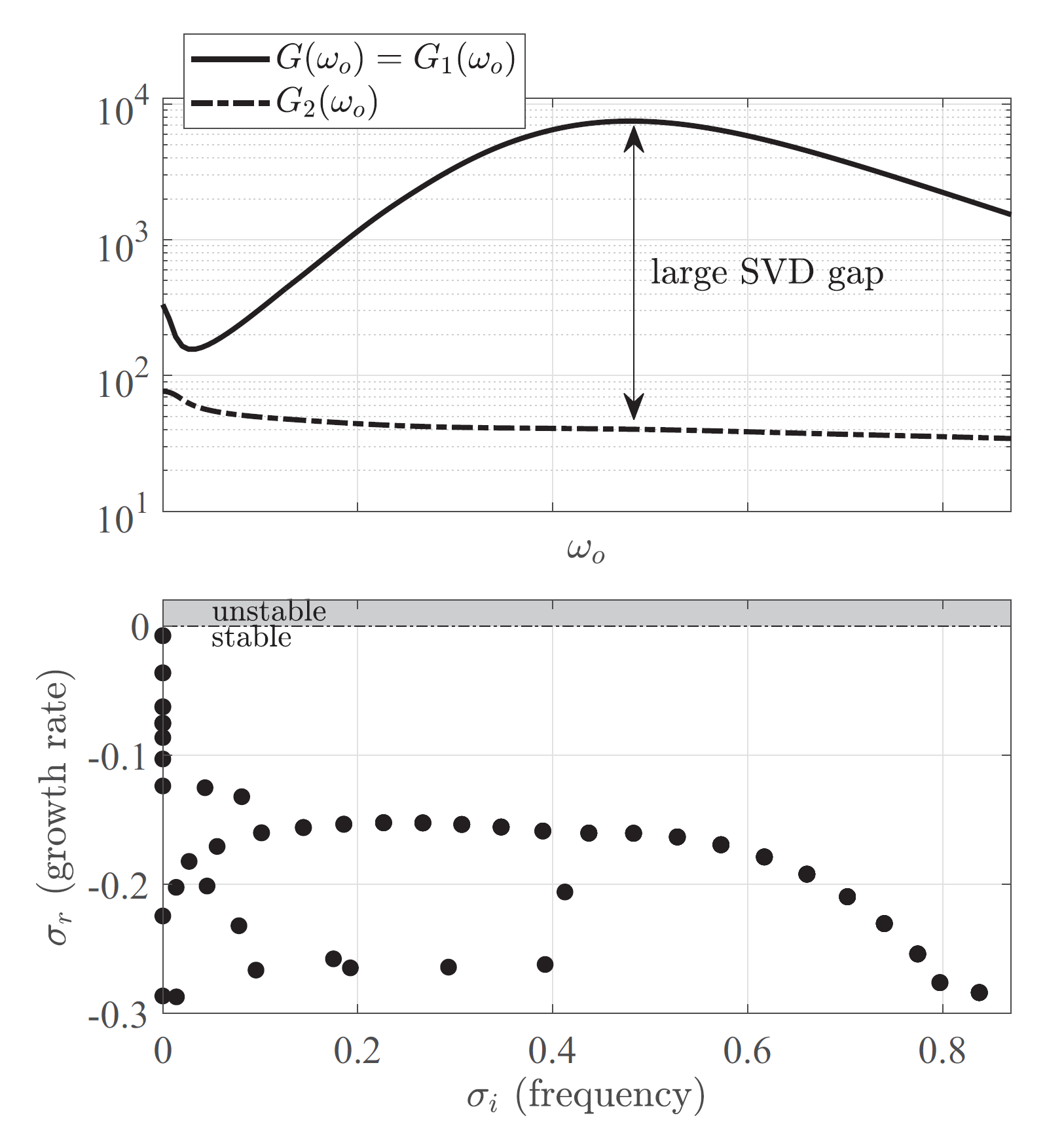
The low-rank property is of central importance! Let us consider, for instance, that, in the equation above, \(G_1 \gg G_2 > ...\), then,

\[\hat{u}_h \approx G_1 \check{u}_1 \langle \check{f}_1 \mid \hat{f}_h \rangle.\]

which means that, for a generic \(\hat{f}_h\), the harmonic response \(\hat{u}_h\) is well approximated by \(\check{u}_1\) alone! In other words, projecting the linear response in the subspace spanned by the few dominant nonmodal responses extracts the leading-order response. In turn, this implies that, at least in the linear regime, it is justified to reduce the Navier-Stokes equations to a low-dimensional system for the coordinates within this subspace.

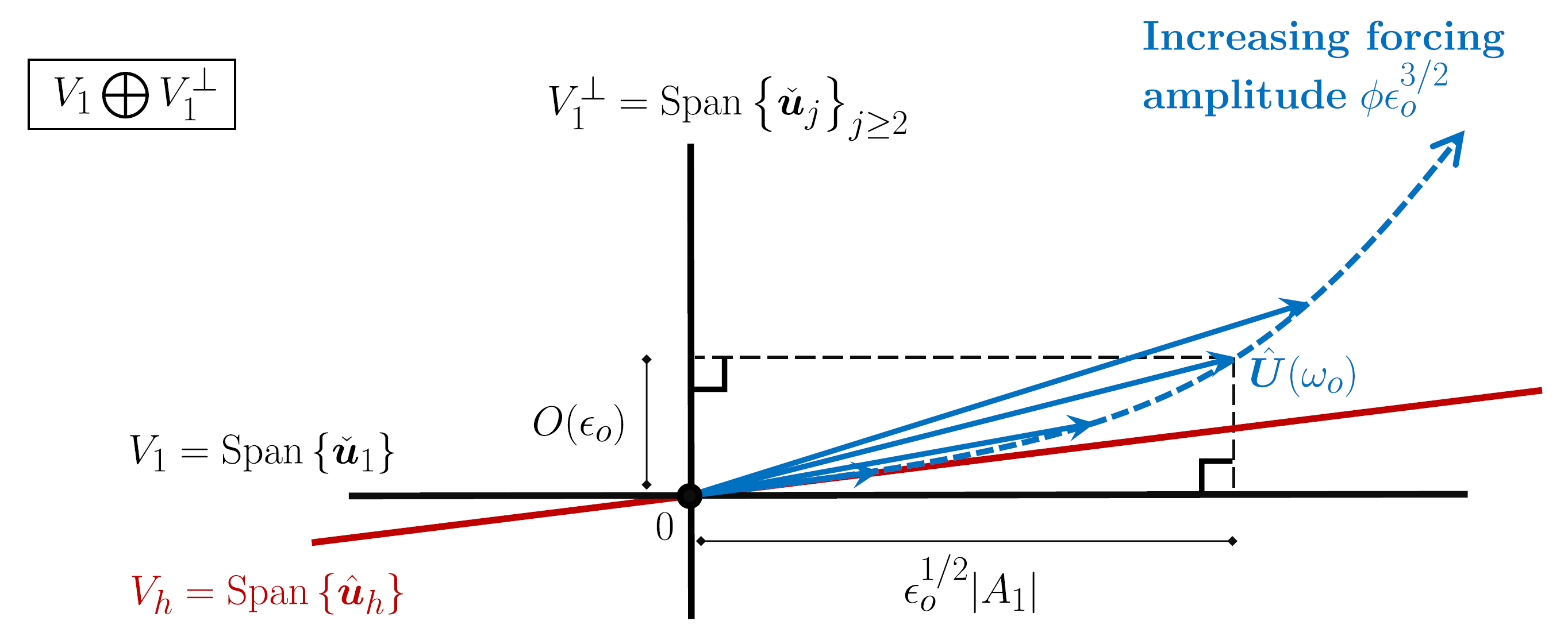
In (Ducimetière & Gallaire, 2025), François and I argue that projecting the flow response in the subspace spanned by the few dominant linear nonmodal responses also extracts the leading-order response in a weakly nonlinear regime (see figure 4).

Figure 4. Schematic representation of the weakly nonlinear harmonic response \( \hat{U}(\omega_o) \) (blue arrows, one for each forcing amplitude) in the phase space. The phase space is shown here in the orthonormal basis formed by the \(\{ \check{u}_j \}_{j\geq 1}\) family. The subspace \(V_h = Span\{ \hat{u}_h \} \), where the linear response \(\hat{u}_h\) to some arbitrary harmonic forcing \(\hat{f}_h\) is represented in red. By hypothesis, the contribution to \(\hat{u}_h\), which is spanned by the suboptimal responses, i.e., in \(V_1^{\perp} = Span\{ \check{u}_j \}_{j\geq 2} \), is much smaller than that along the optimal one \(\check{u}_1 \). Thereby \( V_h \) makes only a small angle with the subspace \(V_1 = Span\{ \check{u}_1 \} \). For vanishing harmonic forcing amplitude, the weakly nonlinear harmonic response must be tangent to \(V_h\). However, as the forcing amplitude is increased, they become increasingly misaligned (please see the evolution of the blue arrows for increasing forcing amplitude). Consequently, as the forcing amplitude is increased, the locus of the weakly nonlinear responses (blue dashed line) is curved in the phase space. Yet, by continuity, the weakly nonlinear response still makes a small angle with the subspace \(V_1\), such that its projection on \( V_1 \) still gives the leading-order response.

Thereby, we could derive a low-dimensional system of equations for the amplitudes of the dominant nonmodal responses, which incorporate the leading-order nonlinearities of the Navier-Stokes equations (They are valid in a regime where the error resulting from neglecting the higher-order nonlinearities is small according to the chosen induced norm.) Owing to their simplicity, such nonmodal amplitude equations were found to bring insight into the weakly nonlinear mechanisms that modify the gains as one increases the amplitude of the initial condition, the harmonic forcing, or a stochastic forcing, respectively.

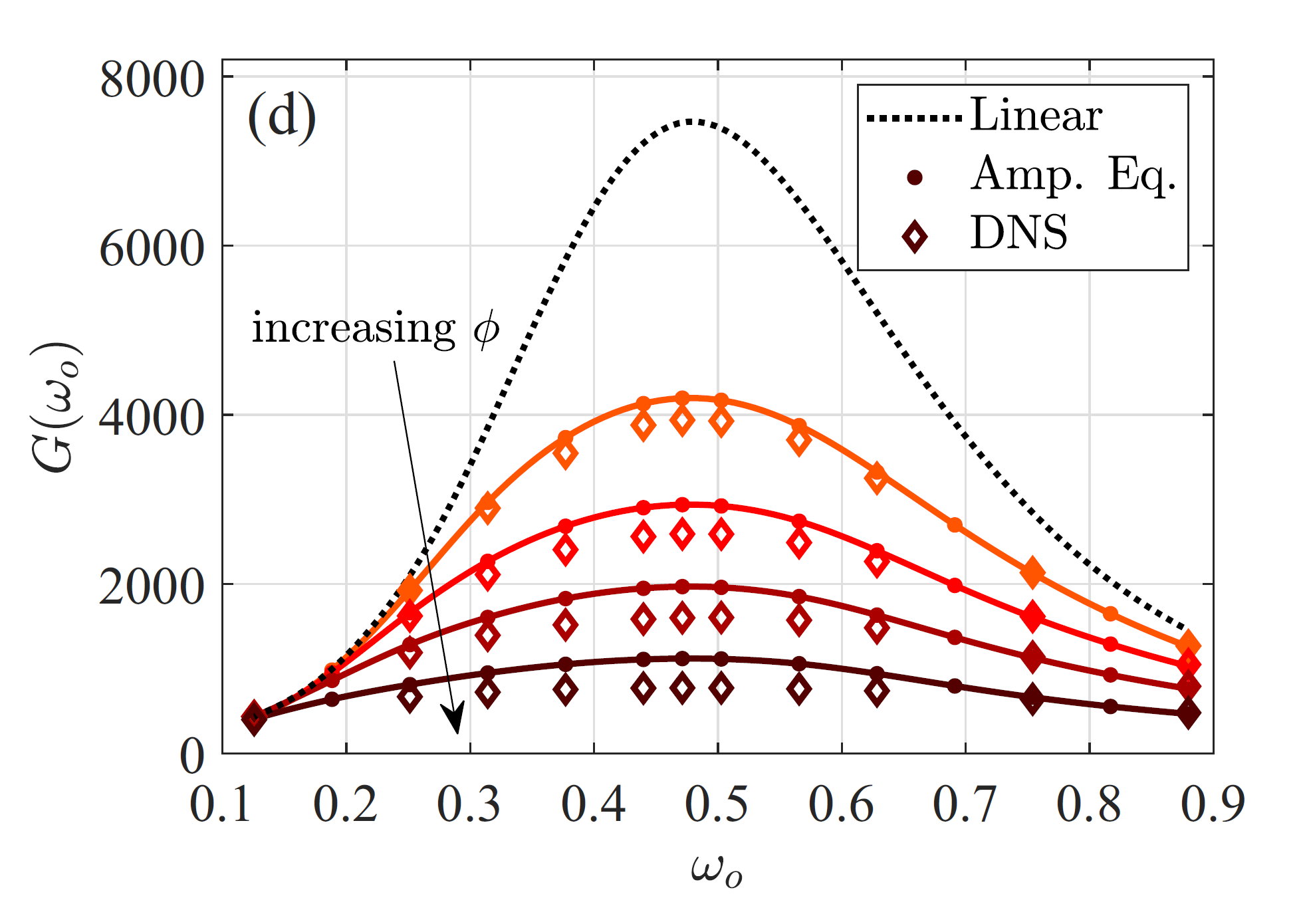
For instance, again considering the response to a harmonic forcing, under the low-rank assumption that \(G_1\gg G_2 > G_3>...\) we could derive in (Ducimetière & Gallaire, 2025) that

\begin{equation} 0 = - A - A|A|^2( \mu + \nu) + \phi \langle \check{f}_1 \mid \hat{f}_h \rangle + h.o.t. , \label{eq:1} \end{equation}

where \(A\) is the amplitude of \(\check{u}_1\) (the leading-order harmonic response) and \(\phi\) the amplitude of the harmonic forcing. Some closed-form analytical expressions were given for the coefficients \(\mu\) and \(\nu\). The equation \eqref{eq:1} contains a non-linear term, such that for sufficiently small forcing amplitude \(\phi\), yet up to values large enough to depart from the linear regime, the amplitude equation can predict the nonlinear evolution of the gain as \(\phi\) is increased (see figure 5).

Figure 5. Harmonic gain for the BFS (see Fig. 2) flow at \( Re=500 \) subjected to the (linear) optimal forcing structure, i.e., \(\hat{f}_h = \check{f}_1\). The gain is obtained from a linear (dotted line), a leading-order weakly nonlinear from (Ducimetière & Gallaire, 2025), and a fully nonlinear (DNS, diamond markers) approach. Darker nuances correspond to larger forcing amplitudes \(\phi\).

With Edouard Boujo , we have also shown in (Ducimetière et al., 2022), (Ducimetière et al., 2022) and (Ducimetière & Gallaire, 2023) that these nonmodal amplitudes equation for the response to a harmonic forcing, a stochastic forcing, and an initial perturbation, respectively, can also be derived using multiple scale asymptotic expansions.
Specifically, we have shown that the inverse of the relevant input/output operator, due to its non-normality, could be made singular with a very small perturbation (as small as \(1/G_1\)), even if the eigenvalues of the original operator all have a large damping rate. The associated kernel is along the optimal response (i.e., the most amplified one, associated with \(G_1\)), since the singularised operator corresponds to the original one projected into the subspace spanned by the sub-optimal responses only. This operator perturbation can be encompassed in an otherwise classical multiple-scale asymptotic expansion, closed by imposing compatibility conditions. Again, the leading order is entirely contained in the optimal subspace, whereas the singularised operator, for the contributions in the sub-optimal one, determines the higher-order fields in the expansion.

But a lot of work remains to be done! I propose below two projects which I am looking forward to working on in the future (my current postdoc is concerned with another topic).

(i) The nonmodal amplitude equations, at least in their current forms (the simplest possible), were found to mostly fail to predict subcritical transitions of the flow as the forcing amplitude was increased to too large values, causing the nonlinear flow response to transit to a state structurally completely different from the linear one. That is because, in our approach, the weakly nonlinear response is sought as an asymptotic expansion where only the optimal response is included at leading order, and thus the former is condemned to remain structurally close to the latter. In other terms, our approach, in its current implementation, has too little freedom over the spatial structure to systematically predict the occurence of subcritical transitions!
While the latter feature is what makes the reduction to a very low-dimensional system possible, it is indeed problematic in the subcritical transition scenario. There, the flow may go into a nonlinear state that is spatially much richer than that around which the expansion is performed. This enrichment may involve many suboptimal structures, but also many additional wave-number pairs (and not just harmonics of the fundamental pair, already included).

(ii) I am hopeful that a precise link between the reduction procedure we have proposed and the parameterization method could be drawn, at least for the harmonic forcing problem. Note that this link is not a priori obvious, for the reduction we have proposed is not performed in an eigensubspace, which, as we have seen, often cannot be chosen low-dimensional and still yield a good description of the nonmodal responses.
In particular, in figure 3, the locus of the weakly nonlinear response (dashed line) might be seen as analogous to a center manifold for the modal paradigm, whereas \(V_h\) would be analogous to the center eigenspace (the former being tangent to the latter in the linear regime). Thereby, adopting, for instance, the graph style of the parameterization method, and seeking the part of the nonlinear correction of solution which is contained in the suboptimals subspace \(V_1^{\perp}\), as a graph over the amplitude along the optimal subspace \(V_1\), could be another manner to derive Eq. \eqref{eq:1}.
Being able to derive the same equation by using the parameterization method would, from a fundamental perspective, possibly make available the subsequent theorem of existence. From a practical implementation one, it would perhaps make possible an automated derivation of the reduced-order systems, which would be extremely useful when including several amplitudes or going to higher orders, for in these two situations, the calculations become quickly tedious to perform by hand.

References

2025

2024

2023

2022